Tag Archives: Neo4j

Options for Structuring Graph Databases

I’d like to start by explaining why I referred to “NOSQL” rather than “NoSQL”: I believe that “Not Only SQL” is more accurate than “No SQL” because, of course, we can make use of both relational databases and the alternatives like document and graph. In fact this is probably just about the most miss-leading terminology of recent years because, as you will see from this article, Graph databases are structured and have query languages so they are in those regards no different to relational databases. Rant over, let me describe what I’ve learnt and hope it of help to your own journey beyond relational databases.

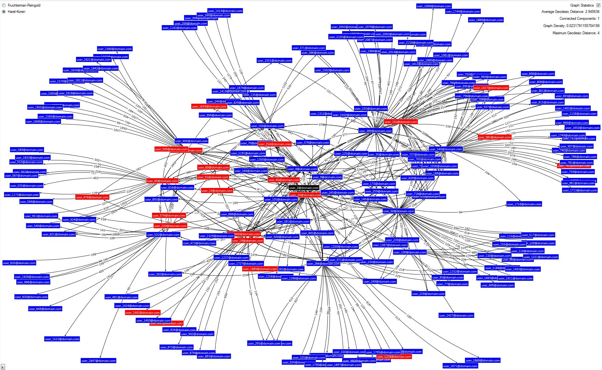
The reason I started working with a Graph database was to help my research into Social/Organisational Network Analysis. To get beyond the basics and start to really understand influence, and how it changes over time, I needed to be able to query the composition and strength of multiple individuals’ networks, enter the Graph Database. I won’t try explaining the concepts of a Graph Database as Wikipedia does an excellent job so I’ll jump straight in assuming you read the Wikipedia article. I chose to use Neo4j because there is some support for .NET via a couple of APIs. For the purposes of this discussion the key constructs in Neo4j are: nodes (vertices), relationships (edges) and attributes; both nodes and edges can have attributes.

The data entities I have been dealing with are: employees and items of electronic communication such as email and IM as well as other pieces of information that help identify the strength of social ties such as corporate directories, project time records and meeting room bookings. There is a whole spectrum of how these can be represented in a Graph Database but I will look at three scenarios I have either implemented, seen implemented or considered.

1)      Everything is a node

graph database 1

All the entities you might have previously placed in a relational database become a node, complete with all the attributes such as “meeting duration”. There are relationships between the nodes which have a type and may also have additional attributes.

Advantages: all the data in one place; you have the flexibility to query the graph in as much detail as the captured attributes allow.

Disadvantages: you could end up with a lot of nodes and relationships, the 2000 person organisation I studied produced well over a million emails per month so by the time you add in IMs and other data over a couple of years you will be in the 100 million plus range for nodes and even more for relationships potentially giving you an actual [big data] problem as opposed to the usual big [data problem]; the queries could be very complex to construct, perhaps not an issue once you have some experience but it might be better to start with something simpler.

2)      Most things are a relationship

graph database 2

Here we keep only the ‘real world’ entities, the people, as nodes and push all the other information into relationships. For my study this would massively reduce the number of nodes but not relationships. In fact for some information, like attendance of a given meeting, the number of edges dramatically increases from n (where n is the number of people in the meeting) to n(n − 1)/2 (a complete graph).

Advantages: a lot fewer nodes (depending on the characteristics of the information involved)

Disadvantages: more edges (depending on the characteristics of the information involved); duplication of attribute information (e.g. meeting duration) in relationships; might make some queries harder or not possible.

3) Hybrid Relational-Graph

graph database 3

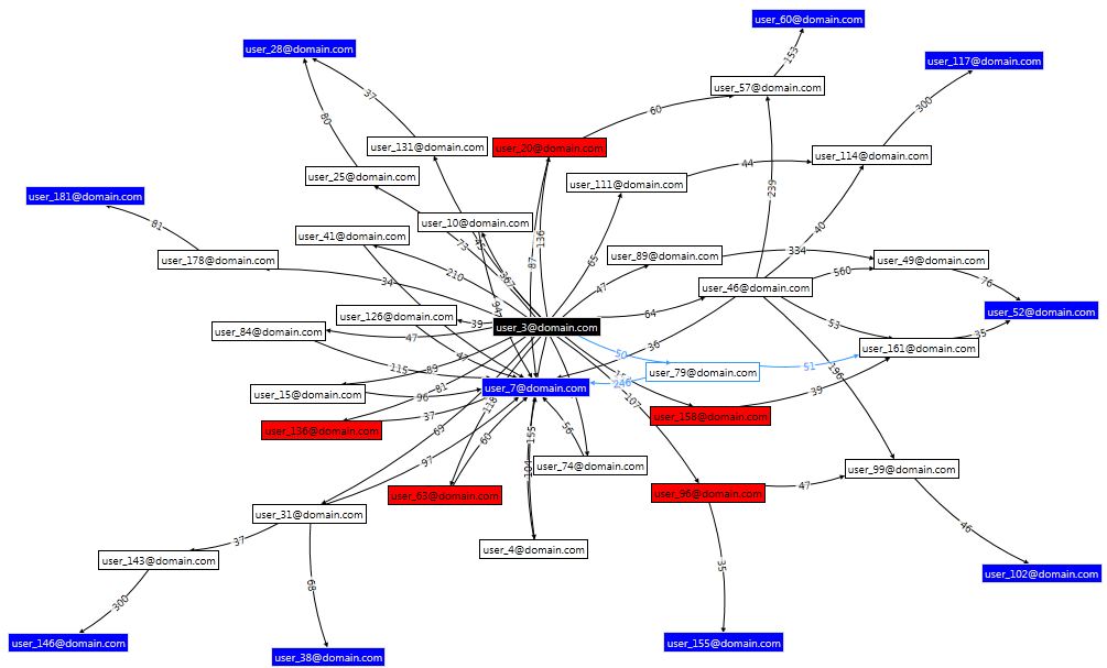
This approach effectively uses the Graph Database as a smart index to the relational data. It was ideal for my Social Network Analysis because I only needed to know the strength of relationship between the people(nodes) so was able to leverage the power of the relational database to generate these using the usual ‘group by’ clauses. I’ve shown an ETL from the Relational data to the Graph data because that’s the flow I used but they could be bi-directional or built in parallel.

Advantages: much smaller graph (depending on the characteristics of the information involved), in my data sets I’ve found 1,000 employees mean around 100,000 relationships; much simpler graph queries.

Disadvantages: Data in two places, which needs to be joined and risks synchronisation problems.

As you can guess I like the third option, mostly because it’s a gentler introduction in terms of simplicity and scale, you are less likely to write queries which attempt to return millions of paths!

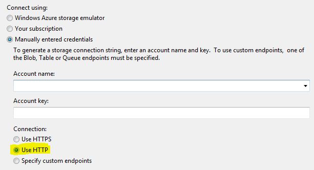
At the beginning (in the rant section) I mentioned Neo4j has a query language (actually it has two). Rather than repeat myself take a look at a previous post where I describe some Cypher queries.


Running Neo4j on Windows Azure

There are a number of approaches to getting Neo4j onto Azure, some of which are listed on the Neo4j’s website. Dynamic Deploy looked like the best approach but for some reason it would not offer deployment to Europe. There are also some pre-built Linux images but I wanted a Windows-based install so that I could easily troubleshoot any problems. Eventually I followed this post which installs Neo4j into an Azure worker role. This really shows what can be done with the PaaS approach, as opposed to using a VM: it installs and configures Java and Neo4j, creates and/or attaches a virtual hard drive and starts Neo4j bound to a custom port. As the author notes this was written against an older version of the SDK. To bring it to the latest version just search out all the references to Azure libraries and change then to the latest version. I also had problems with the VM as it seems the connection can’t be https; I’ve not investigated why this is so for now I’ve changed it, as shown below, to http:

Neo4j Azure Connection String B

The Storage connection string setting should now look like this:

Neo4j Azure Connection String A

And one more thing, you may find firewalls block port 5000 so you could try some commonly allowed ones like 8080.


Calculating Influence

If influence can roughly be equated with the volume, and to whom, an individual communicates then an ‘influencing score’ can be calculated. I’m not looking here at measures of centrality; although I do plan in incorporate this at a later date. Within what appears to be a command-and control organisation rank is very important and is known for each individual. I propose that the influencing score between any two individuals is made from the following three factors:

  • The rank of the target to which the subject is connected
  • The strength of the connection (dictated by the lowest scoring edge)
  • The distance (number of edges) from the subject to the target

It would also be essential to track changes over time is this to be a useful measure.

How did I go about creating this?

  • First I created a scored relationship, as described before, (but reducing the value of being a line manager to 30) between each person (node) on a per-month basis. Each relationship (link) was typed consistently so, for example for May 2013 is called MONTH_2013_05
  • Secondly I use a dynamically generated Cypher query  to obtain the graph (network) of relationships to the subject for each month:  START n=node:node_auto_index(email = ‘[email protected]’) MATCH p = (n)-[:MONTH_2013_05*1..2]-(x) RETURN DISTINCT ‘~’ AS begin, length(p) AS len, EXTRACT( n IN NODES(p):n.email + ‘<‘ + n.rank + ‘>’) AS email, EXTRACT( r IN RELATIONSHIPS(p):r.score) AS score. I won’t pick this query apart here but if anyone wants an explanation please get in touch. I’m also not using any Neo4j client libraries and simply parsing out the result which is why there is a ‘~‘ to mark the start of each record.
  • The score, for each path (the ‘p’ in the Cypher query is then calculated and all the scores are added together. Here is an example:  A—(67)—B—(50)—C<rank 4> where A is the subject  has a score of 50 (the weakest link) * 6 ( the multiplier for rank 4, more later) * 0.1 (the distance factor)

Because rank is considered so important the highest ranks are given much higher multipliers as listed: 0:100, 1:50, 2:25, 3:12, 4:6, 5:3, 6:2, <=7:1

Indirect relationships are reduced to 10% of the score for a direct relationship. The Cypher query only returns a maximum of 1 intermediate node (1..2)

The following chart shows a plot for three individuals who are in a direct line of management; as expected the influencing score drops as the rank drops. The relative scores are also reasonably consistent.

influence1

The next plot shows another direct line management relationship, the senior manager is the same as before. This time it shows a distinct rise in influence of the mid-ranked individual.

influence2

The measurement of influence I have described is fairly crude, for example it bounces around based on when people are on holiday (this can be fixed by using a value averaged over active days) and there is a degree of double-counting (which can be removed by pruning indirect connections when a direct connection exists) however empirically it produces results that reflect reality of individuals known to the author.

An individual’s view of their network

In my previous post I described searching from a number of target nodes (e.g. people that speak German) back to the querying user (node). It’s very simple (probably simpler) to show a person what their network looks like, pretty much in the way any social networking site can. I’ve combined the results from the two following Cypher queries, the first finds friends and the second friends of friends. I’m sure it could all be done in one query (help me Cypher experts):

START n=node:node_auto_index(email = ‘[email protected]’) MATCH p = (n)–(x) RETURN DISTINCT length(p) AS len, EXTRACT( n IN NODES(p):n.email) AS email, EXTRACT( r IN RELATIONSHIPS(p):r.score) AS score

START n=node:node_auto_index(email = ‘[email protected]’) MATCH p = (n)–(x)–(y) RETURN DISTINCT length(p) AS len, EXTRACT( n IN NODES(p):n.email) AS email, EXTRACT( r IN RELATIONSHIPS(p):r.score) AS score

Again the results from these queries is loaded into memory and ordered by the lowest (weakest) edge score in each path and the highest rated are visualised using NodeXL:

Network

The central person (node), whose network is displayed is coloured black and their connections are blue; red nodes are people who have left the organisation – probably not that useful here.

Cutting it down to size – an individual’s view of the graph

Showing someone a graph of where they fit into an organisation along with over 2000 colleagues is simply not practical, not only can’t it all be fitted on a screen at a meaningful level but it’s just going to be a mess of edges (connections).  I previously described loading SNA data first into a relational database and then into Neo4j. The structure I have built in Neo4j is quite simple: a node (person) has a number of attributes including email address and languages which is a list of languages a person speaks (people provide this information to the corporate directory). The edges in Neo4j have a single attribute, score, which attempts to represent the relative strength of the relationship between two people (nodes). The score is derived from a number of data sources I have previously described.

So here’s the scenario I’m looking at: let’s say you need to find someone who speaks German;  the corporate directory can be searched on a number of attributes including language but what if you don’t know any of the people who speak German and you don’t really want to approach people you don’t know. Well this is where your friends of friends might be able to help but how do you know which of you friends may know one of the people who speak German. Well this is perfect territory for graph databases.

To query Neo4j firstly I’ve enabled auto-indexing for the email and languages attributes (along with others); this is done by editing the neo4j.properties file in the conf folder:

neo4j-auto-index

Then, using the Neo4j’s cypher query language execute the following (I’m rather proud of this Cypher query but I’m sure a Cypher expert might be able to put me right):

START
n=node(*), m=node:node_auto_index(email = ‘[email protected]’)
MATCH
p = allShortestPaths( (m)<-[r*..6]->(n) )
WHERE
n.languages =~ ‘(?i).*german.*’
RETURN DISTINCT
length(p) AS len,
EXTRACT( n IN NODES(p):n.email) AS email,
EXTRACT( r IN RELATIONSHIPS(p):r.score) AS score
ORDER BY
length(p)

Let’s take that apart:

  • START: defines two sets of nodes: n is all or any node, m uses the query to locate the node that matches the email address of the user making the query
  • MATCH: the allShortestPaths is a built-in function that does exactly what it says, its argument restricts this to a maximum of six hops and between the two sets identified in the START clause; it returns a list of paths, referred to as p. (A path contains the both nodes and edges, e.g. you get Node1–Edge1->Node2–Edge2->Node3). Every path will connect a node n (the German speaker) to node m (the user making the query) and include up to 4 intermediary nodes.
  • WHERE: this reduces the size of set n (remember this is node(*) ) to only those that have a language attribute matching the supplied regular expression (the fiddly bits just means ignore the case)
  • RETURN: there will be three things returned:
    • the length of the path,
    • a list of all the nodes in the path
    • the ‘score’ values between each pair of nodes
    • ORDER BY: shortest paths are best (usually, more of that next), so the ordering is by the path length

Now shortest paths are best, right? Well maybe but from the work I’ve previously described there is a score for every relationship (edge), is a short path with low scores better than a long path with high scores? Well I don’t know and I’d love to hear from anyone who’s read a paper on the subject or has any views. The following illustrates this, the capital letters represent a node (person) and the number in brackets is the score of the relationship between the two nodes. A is the user making the query and X speaks German, there are the following paths:

Path 1: A–(350)–B–(193)–X

Path 2: A–(5)–C–(9)–X

Path 3: A–(150)–D–(210)–E–(105)–X

Clearly the first is pretty good: the path is short and the relationships are relatively strong. But what about the next one, the path is short but A does not know C that well and, likewise, C does not know X well; it may be better to go via D and E, although the path is longer everyone on it probably has a strong relationship.

Having experimented empirically I found a good result is obtained by ranking the paths based on the lowest relationship score in the path (think of this as the ‘weakest link’), the above three paths are ordered thus (I have highlighted the ‘weakest link’ in each):

Path 1: A–(350)–B–(193)–X

Path 3: A–(150)–D–(210)–E–(105)–X

Path 2: A–(5)–C–(9)–X

Results with this ranking appear to work very well; in general shortest paths tend to feature and longer paths with high scores are rarer because, of course, it only takes one weak link to demote it in the rankings.

The ranked paths can be presented to the user but there is often a lot of redundancy, it could be that Path 3 is repeated but going through node F instead of E. Therefore I’ve found it better to turn the list of paths back into a graph. I’ve used a visualisation component from the excellent NodeXL library to do this. I’ve also limited the number of paths displayed as too many produce a somewhat unreadable result; this is why ranking the paths was important, we want to display the best ones if we can’t display them all.

knows-languages

The black node in the centre is the user making the query; blue nodes are people who can speak German; white nodes are intermediaries. The red nodes represent people who have left the organisation, they aren’t really that useful here I just haven’t got round to adding an option to filter them out. Each relationship (line) is labelled with the score (strength).